9. COMMON PROBABILITY DISTRIBUTIONS

A. Define a probability distribution and distinguish between discrete and continuous random variables and their probability functions :
B. Describe the set of possible outcomes of a specified discrete random variable :
A probability distribution describes the probabilities of all the possible outcomes for a random variable. The probabilities of all possible outcomes must sum to 1.
A discrete random variable is one for which the number of possible outcomes can be counted, and for each possible outcome, there is a measurable and positive probability.
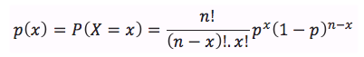
A probability function, denoted p(x), specifies the probability that a random variable is equal to a specific value. More formally, p(x) is the probability that random variable X takes on the value x, or p(x) = P(X=x). The two key properties of a probability function are :
0 ≤ p(x) ≤1.
, the sum of the probabilities for all possible outcomes, x, for a random variable, X, equals 1.
A continuous random variable is one for which the number of possible outcomes is infinite, even if lower and upper bounds exist.
The assignment of probabilities to the possible outcomes for discrete and continuous random variables provides us with discrete probability distributions and continuous probability distributions. The difference between these types of distributions is most apparent for the following properties :
- For a discrete distribution, p(x) =0 when x cannot occur, or p(x) >0 if it can.
- For a continuous distribution, p(x) =0 even though x can occur. We can only consider P(x1 ≤ X ≤ x2) where x1 and x2 are actual numbers.
In finance, some discrete distributions are treated as though they are continuous because the number of possible outcomes is very large.
C. Interpret a cumulative distribution function :
D. Calculate and interpret probabilities for a random variable, given its cumulative distribution function :
A cumulative distribution function (cdf), or simply distribution function, defines the probability that a random variable, X, takes on a value equal to or less than a specific value, x. It represents the sum, or cumulative value, of the probabilities for outcomes up to and including a specified outcome. The cumulative distribution function for a random variable, X, may be expressed as F(x) = P(X ≤ x).
E. Define a discrete uniform random variable, a Bernoulli random variable, and a binomial random variable :
F. Calculate and interpret probabilities given the discrete uniform and the binomial distribution functions :
A discrete uniform random variable is one for which the probabilities for all possible outcomes for a discrete random variable are equal. Also, the cumulative distribution function for the nth outcome, F(xn) = np(x), and the probability for a range of outcomes is p(x)k, where k is the number of possible outcomes in the range.
The Binomial Distribution
A binomial random variable may be defined as the number of “successes” in a given number of trials, whereby the outcome can be either “success” or “failure”. The probability of success, p, is constant for each trial, and trials are independent. A binomial random variable for which the number of trials is 1 is called a Bernoulli random variable. The binomial probability function defines the probability of x successes in n trials and can be expressed using the following formula :
For a given series of n trials, the expected number of successes, or E(X), is given by the following formula : E(X) = np.
The variance of a binomial random variable is given by : Var(X) = np(1 - p).
G. Construct a binomial tree to describe stock price movement :
A binomial model can be applied to stock price movements. We just need to define the two possible outcomes and the probability that each outcome will occur. Consider a stock with current price S that will, over the next period, either increase in value or decrease in value. The possibility of an up-move (the up transition probability, u) is p and the probability for a down move (the down transition probability, d) is (1 – p).
A binomial tree is constructed by showing all the possible combinations of up-moves and down-moves over a number of successive periods. Each of the possible values along a binomial tree is a node.
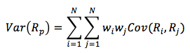
H. Calculate and interpret tracking error :
Tracking error is the difference between the total return on a portfolio and the total return on the benchmark against which its performance is measured.
I. Define the continuous uniform distribution and calculate and interpret probabilities, given a continuous uniform distribution :
The continuous uniform distribution is defined over a range that spans between some lower limit, a, and some upper limit, b, which serve as the parameters of the distribution. Outcomes can only occur between a and b, and since we are dealing with a continuous distribution, even if a < x < b P(X=x)=0. Formally the properties of a continuous uniform distribution may be described as follows :
- For all, a ≤ x1 ≤ x2 ≤ b (for all x1 and x2 between the boundaries a and b).
- P(X < a or X>b) = 0 (the probability of X outside the boundaries is zero).
- P(x1 ≤ X ≤ x2) = (x2 – x1)/(b – a). This defines the probability of outcomes between x1 and x2.
J. Explain the key properties of the normal distribution :
The normal distribution is important for many reasons. Many of the random variables that are relevant to finance and other professional disciplines follow a normal distribution. The normal distribution has the following properties :
- It is completely described by its mean, µ, and variance σ2, stated as X ~ N(µ, σ2). In words, this says that “X is normally distributed with mean µ and variance σ2.
- Skewness = 0, meaning that the normal distribution is symmetric about its mean, so that P(X ≤ µ) = P(µ ≤ X) = 0,5, and mean = median = mode.
- Kurtosis = 3; this is measure of how flat the distribution is.
- A linear combination of normally distributed random variables is also normally distributed.
- The probabilities of outcomes further above and below the mean get smaller and smaller but do not get to zero.
K. Distinguish between a univariate and a multivariate distribution, and explain the role of correlation in the multivariate normal distribution :
Up to this point, our discussion has been strictly focused on univariate distributions, i.e., the distribution of a single random variable.
A multivariate distribution specifies the probabilities associated with a group of random variables and is meaningful only when the behavior of each random variable in the group is in some way dependent upon the behavior of the others. Both discrete and continuous random variables can have multivariate distributions. Multivariate distributions between two discrete random variables are described using joint probability tables. For continuous random variables, a multivariate normal distribution may be used to describe them if all of the individual variables follow a normal distribution. As previously mentioned, one of the characteristics of a normal distribution is that a linear combination of normally distributed random variables is normally distributed as well.
The Role of Correlation in the Multivariate Normal Distribution
Similar to a univariate normal distribution, a multivariate normal distribution can be described by the mean and variance of the individual random variables. Additionally, it is necessary to specify the correlation between the individual pairs of variables when describing a multivariate distribution from a univariate normal distribution.
Using asset returns as our random variables, the multivariate normal distribution for the returns on n assets can be completely defined by the following three sets of parameters :
- n means of the n series of returns (µ1, µ2, …, µn).
- n variances of the n series of returns (σ12, σ22, …,σn2).
- 0,5n(n – 1) pair-wise correlations.
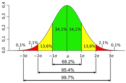
A confidence interval is a range of values around the expected outcome within which we expect the actual outcome to be some specified percentage of the time. A 95% confidence interval is a range that we expect the random variable to be in 95% of the time. Confidence intervals for a normal distribution as illustrated below :
In practice, we will not know the actual values for the mean and standard deviation of the distribution, but will have estimated them as and s. The three confidence intervals of most interest are given by :
- The 90% confidence interval for X is X – 1,65s to X + 1,65s.
- The 95% confidence interval for X is X – 1,96s to X + 1,96s
- The 99% confidence interval for X is X – 2,58s to X + 2,58s
N. Define the standard normal distribution, explain how to standardize a random variable, and calculate and interpret probabilities using the standard normal distribution :
The standard normal distribution is a normal distribution that has been standardized so that it has a mean of zero and a standard deviation of 1. To standardize an observation from a given normal distribution, the z-value of the observation must be calculated. The z-value represents the number of standard deviations a given observation is from the population mean. Standardization is the process of converting an observed value for a random variable to its z-value. The following formula is used to standardize a random variable :
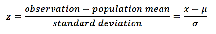
The z-table contains values generated using the cumulative density function for a standard normal distribution, denoted by F(Z). The values in the z-table are the probabilities of observing a z-value that is less than a given value, z (P(Z< z)). From the symmetry of the standard normal distribution, F(-Z) = 1 – F(Z).
O. Define shortfall risk, calculate the safety-first ratio, and select an optimal portfolio using Roy’s safety-first criterion :
Shortfall risk is the probability that a portfolio value or return will fall below a particular value or return over a given time period.
Roy’s safety-first criterion states that the optimal portfolio minimizes the probability that the return of the portfolio falls below some minimum acceptable level. This minimum acceptable level is called the threshold level. Symbolically, Roy’s safety first criterion can be stated as :
Minimize P(Rp < RL)
where
Rp = Portfolio return
RL = threshold level return
If portfolio returns are normally distributed, then Roy’s safety first criterion can be stated as :
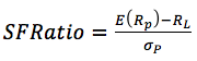
Maximize the SFRatio where :
In summary, when choosing among portfolios with normally distributed returns using Roy’s safety-first criterion, there are two steps :
- Step 1 : Calculate the SFRatio.
- Step 2 : Choose the portfolio that has the larget SFRatio.
P. Explain the relationship between normal and lognormal distributions and why the lognormal distribution is used to model asset prices :
The lognormal distribution is generated by the function ex, where x is normally distributed. Since the natural logarithm, ln, of ex is x, the logarithms of lognormally distributed random variables are normally distributed, thus the name.
The lognormal distribution is skewed to the right.
The lognormal distribution is bounded from below by zero so that it is useful for modeling asset prices which never take negative values.
P. Distinguish between discretely and continuously compounded rates of return, and calculate and interpret a continuously compounded rate of return, given a specific holding period return :
Discretely compounded returns are just the compound returns we are familiar with, given some discreet compounding period, such as semiannual or quarterly. Recall that the more frequent the compounding, the greater the effective annual return.
The effective annual rate, based on a continuous compounding for a stated annual rate of Rcc, can be calculated from the formula :
effective annual rate = EAR = eRcc – 1 and Rcc = ln(EAR + 1)
One property of continuously compounded rates of return is that they are additive for multiple periods. Note that the effective holding period over two years is calculated by doubling the continuously compounded annual rate. The effective holding period return over T years is given by :
HPRT = eRcc * T – 1
Q. Explain the Monte Carlo simulation and describe its applications and limitations :
Monte Carlo simulation is a technique based on the repeated generation of one of more risk factors that affect security values, in order to generate a distribution of security values. For each of the risk factors, the analyst must specify the parameters of the probability distribution that the risk factor is assumed to follow. A computer is then used to generate random values for each risk factor based on its assumed probability distributions. Each set of randomly generated risk factors is used with a pricing model to value the security. This procedure is repeated many times (100s, 1000s, or 10000s), and the distribution of simulated asset values is used to draw inferences about the expected (mean) value of the security and possibly the variance of security values about the mean as well.
Monte Carlo simulation is used to :
- Value complex securities.
- Simulate the profits/losses from a trading strategy.
- Calculate estimates of value at risk (VAR) to determine the riskiness of a portfolio of assets and liabilities.
- Simulate pension fund assets and liabilities over time to examine the variability of the difference between the two.
- Value portfolios of assets that have non-normal returns distributions.
The limitations of Monte Carlo simulation are that it is fairly complex and will provide answers that are no better than the assumptions about the distributions of the risk factors and the pricing/valuation model that is used. Also, simulation is not an analytic method, but a statistical one, and cannot provide the insights that analytical methods can.
R. Compare Monte Carlo simulation and historical simulation :
Historical simulation is based on actual changes in value or actual changes in risk factors over some prior period. Rather than model the distribution of risk factors, as in Monte Carlo simulation, the set of all changes in the relevant risk factors over some prior period is used. Each iteration of the simulation involves randomly selecting one of these past changes for each risk factor and calculating the value of the asset or portfolio in question, based on those changes in risk factors.
Historical simulation has the advantage of using the actual distribution of risk factors so that the distribution of changes in the risk factors does not have to be estimated. It suffers from the fact that past changes in risk factors may not be a good indication of future changes. Events that occur infrequently may not be a good indication of future changes. Events that occur infrequently may not be reflected in historical simulation results unless the events occurred during the period from which the values for risk factors are drawn. An additional limitation of historical simulation is that it cannot address the sort of “what if” questions that Monte Carlo simulation can.
|
|
