37. Cost of capital
A. Weighted Average Cost of Capital (WACC) :
B. Tax effects on the cost of capital :
The capital budgeting process involves discounted cash flow analysis. To conduct such analysis, you must know the firm’s proper discount rate. The discount rate is the firm’s weighted average cost of capital (WACC) and is also referred to as the marginal cost of capital (MCC).
On the right side of a firm’s balance sheet, we have debt, preferred stock, and common equity. These are normally referred to as the capital components of the firm. Any increase in a firm’s total assets will have to be financed through an increase in at least one of these capital accounts. The cost of each of these components is called component cost of capital :
kd : The rate at which the firm can issue new debt. This is the yield to maturity on existing debt. This is also called the before-tax component cost of debt.
kd.(1 – t) : The after-tax cost of debt. Here, t is the firm’s marginal tax rate. The after-tax component cost of debt, kd.(1 – t), is used to calculate the WACC.
kps : The cost of preferred stock.
kce : The cost of common equity. It is the required return on common stock and is generally difficult to estimate.
In many countries, the interest paid on corporate debt is tax deductible. Because we are interested in the after-tax cost of capital, we adjust the cost of debt, kd, for the firm’s marginal tax rate, t. Because there is typically no tax deduction allowed for payments to common or preferred stockholders, there is no equivalent deduction to kps or kce.
Each investment decision must be made assuming a WACC, which includes each of the different sources of capital and is based on the long-run target weights. A company creates value by producing a return on assets that is higher than the required return on the capital needed to fund those assets.
Because a firm’s WACC reflects the average risk of the projects that make up the firm, it is not appropriate for evaluating all new projects. It should be adjusted upward for projects with greater-than-average risk and downward for projects with less-than-average risk.
The WACC is given by :
WACC = (wd).(kd.(1 – t)) + (wps).(kps) + (wce).(kce)
where:
wd : percentage of debt in the capital structure.
wps : percentage of preferred stock in the capital structure.
wce : percentage of common stock in the capital structure.
C. Alternative methods of calculating the weights used in the WACC :
The weights in the calculation of WACC should be based on the firm’s target capital structure; that is, the proportion (based on market values) of debt, preferred stock, and equity that the firm expects to achieve over time. In the absence of any explicit information about a firm’s target capital structure from the firm itself, an analyst may simply use the firm’s current capital structure (based on market value) or the average capital structure in the firm’s industry, as the best indication of its target capital structure.
D. Optimal capital budget :
A firm’s marginal cost of capital increases as it needs to raise larger amounts of capital. This is shown by an upward-sloping marginal cost of capital curve.
An investment opportunity schedule shows the IRRs of (in decreasing order), and the initial amounts for, a firm’s potential projects.
The intersection of a firm’s investment opportunity schedule with its marginal cost of capital curve indicates the optimal amount of capital expenditure, the amount of investment required to undertake all positive NPV projects.
E. The marginal cost of capital’s role in determining the NPV of a project :
All projects do not have the same risk. The WACC is the appropriate discount rate for projects that have approximately the same level of risk as the firm’s existing projects. This is because the component costs of capital used to calculate the firm’s WACC are based on the existing level of firm risk. To evaluate a project with greater than (the firm’s) average risk, a discount rate greater than the firm’s existing WACC should be used. Projects with below-average risk should be evaluated using a discount rate less than the firm’s WACC.
An additional issue to consider when using a firm’s WACC to evaluate a specific project is that there is an implicit assumption that the capital structure of the firm will remain at the target capital structure over the life of the project.
F. Calculating the cost of fixed rate debt :
The after-tax cost of debt, kd.(1 – t), is used in computing the WACC. It is the interest rate at which firms can issue new debt (kd) net of the tax savings from the tax deductibility of interest, kd.(t) :
after-tax cost of debt = interest rate – tax savings = kd - kd.(t) = kd.(1 - t)
The Yield-To-Maturity (YTM) approach assumes the before-tax cost of debt capital is the YTM on the firm’s existing publicly traded debt.
If a market YTM is not available because the firm’s debt is not publicly traded, the analyst can use the debt rating approach, estimating the before-tax cost of debt capital based on market yields for debt with the same rating and average maturity as the firm’s existing debt.
G. Calculating the cost of noncallable, nonconvertible preferred stock :
The cost of preferred stock (kps) is :
kps = Dps / P
where:
Dps = preferred dividends.
P = market price of preferred.
H. Calculating the cost of common equity :
The opportunity cost of common equity capital (kce) is the required rate of return on the firm’s common stock. The rationale here is that the firm could avoid part of the cost of common stock outstanding by using retained earnings to buy back shares of its own stock. The cost of common equity can be estimated using one of the following three approaches :
1. The capital asset pricing model (CAPM) approach :
Step 1 : Estimate the risk-free rate, RFR. Yields on default risk-free debt such as U.S. Treasury notes are usually used. The most appropriate maturity to choose is one that is close to the useful life of the project.
Step 2 : Estimate the stock’s beta, β. This is the stock’s risk measure.
Step 3 : Estimate the expected rate of return on the market E(Rm).
Step 4 : Use the capital asset pricing model (CAPM) equation to estimate the required rate of return :
kce = RFR + β . (E(Rm) – RFR)
2. The dividend discount model approach :
If dividends are expected to grow at a constant rate, g, then the current value of the stock is given by the dividend growth model:

where :
D1 = next year’s dividend
kce = required rate of return on common equity
g = firm’s expected constant growth rate
Rearranging the terms, you can solve for kce :
D1 = next year’s dividend
kce = required rate of return on common equity
g = firm’s expected constant growth rate
Rearranging the terms, you can solve for kce :

In order to use the formula, you have to estimate the expected growth rate, g. This can be done by :
g = (retention rate).(return on equity) = (1 – payout rate).(ROE)
3. Bond yield plus risk premium :
Analyst often use an ad hoc approach to estimate the required rate of return. They add a risk premium (3 to 5 percentage points) to the market yield on the firm’s long-term debt.
kce = bond yield + risk premium
I. Calculating the beta and cost of capital for a project :
A project’s beta is a measure of its systematic or market risk. Just as we can use a firm’s beta to estimate its required return on equity, we can use a project’s beta to adjust for differences between a specific project’s risk and the average risk of a firm’s projects.
Because a specific project is not represented by a publicly traded security, we typically cannot estimate a project’s beta directly. One process that can be used is based on the equity beta of a publicly traded firm that is engaged in a business similar to, and with risk similar to, the project under consideration. This is referred to as the pure-play method.
The beta of a firm is a function not only of the business risks of its projects (lines of business) but also of its financial structure. For a given set of projects, the greater a firm’s reliance on debt financing, the greater its equity beta. For this reason, we must adjust the pure-play beta from a comparable company (or group of companies) for the company’s leverage (unlever it) and then adjust it (re-lever it) based on the financial structure of the company evaluating the project. We can then use the equity beta to calculate the cost of equity to be used in evaluating the project.
To get the asset beta for a publicly traded firm, we use the following formula :
- Using the growth rate as projected by security analysts.
- Using the following equation to estimate a firm’s sustainable growth rate :
g = (retention rate).(return on equity) = (1 – payout rate).(ROE)
3. Bond yield plus risk premium :
Analyst often use an ad hoc approach to estimate the required rate of return. They add a risk premium (3 to 5 percentage points) to the market yield on the firm’s long-term debt.
kce = bond yield + risk premium
I. Calculating the beta and cost of capital for a project :
A project’s beta is a measure of its systematic or market risk. Just as we can use a firm’s beta to estimate its required return on equity, we can use a project’s beta to adjust for differences between a specific project’s risk and the average risk of a firm’s projects.
Because a specific project is not represented by a publicly traded security, we typically cannot estimate a project’s beta directly. One process that can be used is based on the equity beta of a publicly traded firm that is engaged in a business similar to, and with risk similar to, the project under consideration. This is referred to as the pure-play method.
The beta of a firm is a function not only of the business risks of its projects (lines of business) but also of its financial structure. For a given set of projects, the greater a firm’s reliance on debt financing, the greater its equity beta. For this reason, we must adjust the pure-play beta from a comparable company (or group of companies) for the company’s leverage (unlever it) and then adjust it (re-lever it) based on the financial structure of the company evaluating the project. We can then use the equity beta to calculate the cost of equity to be used in evaluating the project.
To get the asset beta for a publicly traded firm, we use the following formula :

where:
D/E = comparable company’s debt-to-equity ratio and t is its marginal tax rate.
To get the equity beta for the project, we use the subject firm’s tax rate and debt-to equity ratio :
D/E = comparable company’s debt-to-equity ratio and t is its marginal tax rate.
To get the equity beta for the project, we use the subject firm’s tax rate and debt-to equity ratio :

While the method is theoretically correct, there are several challenging issues involved in estimating the beta of comparable (or any) company’s equity :
J. Country equity risk premium :
Using the CAPM to estimate the cost of equity is problematic in developing countries because beta does not adequately capture country risk. To reflect the increased risk associated with investing in a developing country, a country risk premium is added to the market risk premium when using the CAPM.
The revised CAPM equation is stated as :
kce = RFR + β . (E(Rm) – RFR + CRP)
where:
CRP = country risk premium
The general risk of the developing country is reflected in its sovereign yield spread. This is the difference in yields between the developing country’s government bonds and Treasury bonds of a similar maturity.
The country risk premium for a developing country can be estimated as the spread between the developing country’s sovereign debt (denominated in a developed country’s currency) and the developed country’s sovereign debt (U.S. Treasury Bills ...), multiplied by the ratio of the volatility of the developing country’s equity market to the volatility of the market for its developed-country-denominated sovereign debt.
K. Marginal cost of capital schedule and break points :
The marginal cost of capital (MCC) is the cost of the last new dollar of capital a firm raises. As firm raises more and more capital, the costs of different sources of financing will increase. Issuing new equity is more expensive than using retained earnings due to flotation costs. The bottom line is that raising additional capital results in an increase in the WACC.
The marginal cost of capital schedule shows the WACC for different amounts of financing. Typically, the MCC is shown as a graph. Because different sources of financing become more expensive as the firm raises more capital, the MCC schedule typically has an upward slope.
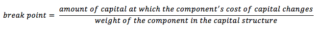
Break points occur any time the cost of one of the components if the company’s WACC changes. A break point is calculated as:
- Beta is estimated using historical returns data. The estimate is sensitive to the length of time and the frequency of the data.
- The estimate is affected by which index is chosen to represent the market return.
- Betas are believed to revert toward 1 over time, and the estimate may need to be adjusted for this tendency.
- Estimates of beta for small- capitalization firms may need to be adjusted upward to reflect risk inherent in small firms that is not captured by the usual estimation methods.
J. Country equity risk premium :
Using the CAPM to estimate the cost of equity is problematic in developing countries because beta does not adequately capture country risk. To reflect the increased risk associated with investing in a developing country, a country risk premium is added to the market risk premium when using the CAPM.
The revised CAPM equation is stated as :
kce = RFR + β . (E(Rm) – RFR + CRP)
where:
CRP = country risk premium
The general risk of the developing country is reflected in its sovereign yield spread. This is the difference in yields between the developing country’s government bonds and Treasury bonds of a similar maturity.
The country risk premium for a developing country can be estimated as the spread between the developing country’s sovereign debt (denominated in a developed country’s currency) and the developed country’s sovereign debt (U.S. Treasury Bills ...), multiplied by the ratio of the volatility of the developing country’s equity market to the volatility of the market for its developed-country-denominated sovereign debt.
K. Marginal cost of capital schedule and break points :
The marginal cost of capital (MCC) is the cost of the last new dollar of capital a firm raises. As firm raises more and more capital, the costs of different sources of financing will increase. Issuing new equity is more expensive than using retained earnings due to flotation costs. The bottom line is that raising additional capital results in an increase in the WACC.
The marginal cost of capital schedule shows the WACC for different amounts of financing. Typically, the MCC is shown as a graph. Because different sources of financing become more expensive as the firm raises more capital, the MCC schedule typically has an upward slope.
Break points occur any time the cost of one of the components if the company’s WACC changes. A break point is calculated as:
L. Correct treatment of flotation costs :
Flotation costs are the fees charged by investment bankers when a company raises external capital. Flotation costs can be substantial and often amount to between 2% and 7% of the total amount of equity capital raised, depending on the type of offering.
In the incorrect treatment, flotation costs effectively increase the WACC by a fixed percentage and will be a factor for the duration of the project because future project cash flows are discounted at this higher WACC to determine project NPV. The problem with this approach is that flotation costs are not an ongoing expense for the firm. Flotation costs are a cash outflow that occurs at the initiation of a project and affect the project NPV by increasing the initial cash outflow. Therefore, the correct way to account for flotation costs is to adjust the initial project cost. An analyst should calculate the dollar amount of the flotation cost attributable to the project and increase the initial cash outflow for the project.
|
|
