7. STATISTICAL CONCEPTS AND MARKET RETURNS
A. Distinguish between descriptive statistics and inferential statistics, between a population and a sample, and among the types of measurement scales :
Statistical methods fall into one of two categories :
- Descriptive statistics are used to summarize the important characteristics of large data sets.
- Inferential statistics pertain to the procedures used to make forecasts, estimates, or judgments about a large set of data on the basis of the statistical characteristics of a smaller set.
A population is defined as the set of all possible members of a stated group. It is frequently too costly or time consuming to obtain measurements for every member of a population, if it is even possible. In this case, a sample may be used. A sample is defined as a subset of the population of interest. Once a population has been defined, a sample can be drawn from the population, and the sample’s characteristics can be used to describe the population as a whole.
Measurement scales may be classified into one of four major categories :
- Nominal scales. Nominal scales are the level of measurement that contains the least information. Observations are classified or counted with no particular order.
- Ordinal scales. Ordinal scales represent a higher level of measurement than nominal scales. When working with an ordinal scale, every observation is assigned to one of several categories. Then these categories are ordered with respect to a specified characteristic.
- Interval scales. Interval scale measurements provide relative ranking, like ordinal scales, plus the assurance the differences between scale values are equal.
- Ratio scales. Ratio scales represent the most refined level of measurement. Ratio scales provide ranking and equal differences between scale values, and they also have a true zero point as the origin.
B. Define a parameter, a sample statistic, and a frequency distribution :
A measure used to describe a characteristic of a population is referred to as a parameter. While many population parameters exist, investment analysis usually utilizes just a few, particularly mean return and the standard deviation of returns.
In the same manner that a parameter may be used to describe a characteristic of a population, a sample statistic is used to measure a characteristic of a sample.
A frequency distribution is a tabular presentation of statistical data that aids the analysis of large data sets. Frequency distributions summarize statistical data by assigning it to specified groups, or intervals. Also, the data employed with a frequency distribution may be measured using any type of measurement scale. The following procedure describes how to construct a frequency distribution :
- Step 1 : Define the interval.
- Step 2 : Tally the observations.
- Step 3 : Count the observations.
C. Calculate and interpret relative frequencies and cumulative relative frequencies, given a frequency distribution :
The relative frequency is calculated by dividing the absolute frequency to each return interval by the total number of observations. Simply stated, relative frequency is the percentage of total observations falling within each interval.
Ii is also possible to compute cumulative absolute frequency and cumulative relative frequency by summing the absolute or relative frequencies starting at the lowest interval and progressing through the highest.
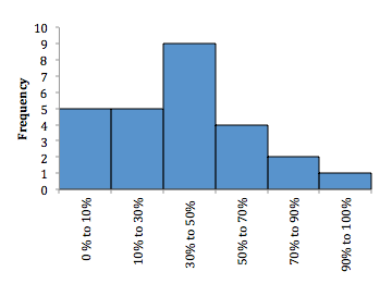
D. Describe the properties of a data set presented as a histogram or a frequency polygon :
A histogram is the graphical presentation of the absolute frequency distribution. A histogram is simply a bar chart of continuous data that has been classified into a frequency distribution.
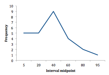
To construct a frequency polygon, the midpoint of each interval is plotted on the horizontal axis, and the absolute frequency for that interval is plotted on the vertical axis. Each point is then connected with a straight line.
E. Calculate and interpret measures of central tendency, including the population mean, sample mean, arithmetic mean, weighted average mean, geometric mean, harmonic mean, median and mode :
Measures of central tendency identify the center, or average, of a data set. This central point can be used to represent the typical, or expected, value in the data set.
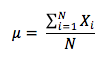
To compute the population mean, all the observed values in the population are summed and divided by the number of observations in the population. Note that the population mean is unique in that a given population only has one mean. The population mean is expressed as :
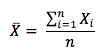
The sample mean is expressed as :
Measures of central tendency identify the center, or average, of a data set. This central point can be used to represent the typical, or expected, value in the data set.
To compute the population mean, all the observed values in the population are summed and divided by the number of observations in the population. Note that the population mean is unique in that a given population only has one mean. The population mean is expressed as :
The sample mean is expressed as :
The population mean and sample mean are both examples of arithmetic means. It is the most widely used measure of central tendency and has the following properties :
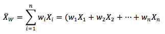
The computation of a weighted mean recognizes that different observations may have a disproportionate influence on the mean. The weighted mean of a set of numbers is computed with the following equation :
where :
X1, X2, …, Xn = observed values
w1, w2, …, wn = corresponding weights associated with each of the observations such that the sum of them all is equal to zero.
The median is the midpoint of a data set when the data is arranged in ascending or descending order. Half the observations lie above the median and half are below. The median is important because the arithmetic mean can be affected by extremely large or small values.
The mode is the value that occurs most frequently in a data set. A data set may have more than one mode or even no mode. When a distribution has one value that appears most frequently, it is said to be unimodal. When a set of data has two or three values that occur most frequently, it is said to be bimodal or trimodal, respectively.
The geometric mean is often used when calculating investment returns over multiple periods or when measuring compound growth rates. The general formula for the geometric mean, G, is a follows :
- All interval and ratio data sets have an arithmetic mean.
- All data values are considered and included in the arithmetic mean computation.
- A data set has only one arithmetic mean.
The computation of a weighted mean recognizes that different observations may have a disproportionate influence on the mean. The weighted mean of a set of numbers is computed with the following equation :
where :
X1, X2, …, Xn = observed values
w1, w2, …, wn = corresponding weights associated with each of the observations such that the sum of them all is equal to zero.
The median is the midpoint of a data set when the data is arranged in ascending or descending order. Half the observations lie above the median and half are below. The median is important because the arithmetic mean can be affected by extremely large or small values.
The mode is the value that occurs most frequently in a data set. A data set may have more than one mode or even no mode. When a distribution has one value that appears most frequently, it is said to be unimodal. When a set of data has two or three values that occur most frequently, it is said to be bimodal or trimodal, respectively.
The geometric mean is often used when calculating investment returns over multiple periods or when measuring compound growth rates. The general formula for the geometric mean, G, is a follows :
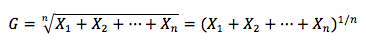
Note that this equation has a solution only if the product under the radical sign is non-negative. Also, when calculating the geometric mean for a returns data set, it is necessary to add 1 to each value under the radical sign and then subtract 1 from the result.
The geometric mean is always less than or equal to the arithmetic mean, and the difference increases as the dispersion of the observations increases.
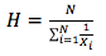
A harmonic mean is used for certain computations, such as the average cost of shares purchased over time. The harmonic mean is calculated as :
where there are N values of Xi.
For values that are not all equal : harmonic mean < geometric mean < arithmetic mean. This mathematical fact is the basis for the claimed benefit of purchasing the same dollar amount of mutual fund shares each month or each week.
F. Calculate and interpret quartiles, quintiles, deciles, and percentiles :
Quantile is the general term for a value at or below which a stated proportion of the data in a distribution lies. Examples of quantiles include :
Note that any quantile may be expressed as a percentile. For example, the third quartile partitions the distribution at a value such that three-fourths, or 75%, of the observations fall below that value. Thus, the third quartile is 75th percentile.
The formula for the position of the observation at a given percentile, y, with n data points sorted in ascending order is :
Ly = (n + 1) (y/100)
Quantiles and measures of central tendency are known collectively as measures of location.
G. Calculate and interpret 1) a range and a mean absolute deviation and 2) the variance and standard deviation of a population and of a sample :
Dispersion is defined as the variability around the central tendency.
The range is relatively simple measure of variability, but when used with other measures it provides extremely useful information : range = maximum value – minimum value.
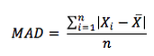
The mean absolute deviation is the average of the absolute values of the deviations of individual observations from the arithmetic mean.
The geometric mean is always less than or equal to the arithmetic mean, and the difference increases as the dispersion of the observations increases.
A harmonic mean is used for certain computations, such as the average cost of shares purchased over time. The harmonic mean is calculated as :
where there are N values of Xi.
For values that are not all equal : harmonic mean < geometric mean < arithmetic mean. This mathematical fact is the basis for the claimed benefit of purchasing the same dollar amount of mutual fund shares each month or each week.
F. Calculate and interpret quartiles, quintiles, deciles, and percentiles :
Quantile is the general term for a value at or below which a stated proportion of the data in a distribution lies. Examples of quantiles include :
- Quartiles – the distribution is divided into quarters.
- Quintile – the distribution is divided into fifths.
- Decile – the distribution is divided into tenths.
- Percentile – the distribution is divided into hundreths (percents).
Note that any quantile may be expressed as a percentile. For example, the third quartile partitions the distribution at a value such that three-fourths, or 75%, of the observations fall below that value. Thus, the third quartile is 75th percentile.
The formula for the position of the observation at a given percentile, y, with n data points sorted in ascending order is :
Ly = (n + 1) (y/100)
Quantiles and measures of central tendency are known collectively as measures of location.
G. Calculate and interpret 1) a range and a mean absolute deviation and 2) the variance and standard deviation of a population and of a sample :
Dispersion is defined as the variability around the central tendency.
The range is relatively simple measure of variability, but when used with other measures it provides extremely useful information : range = maximum value – minimum value.
The mean absolute deviation is the average of the absolute values of the deviations of individual observations from the arithmetic mean.
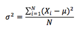
The population variance is defined as the average of the squared deviations from the mean. The population variance is calculated using the following formula :
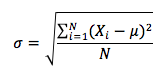
The population standard deviation is the square root of the population variance and is calculated as follows :
The population standard deviation is the square root of the population variance and is calculated as follows :
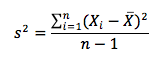
The sample variance is the measure of a dispersion that applies when evaluating a sample of n observations from a population. The sample variance is calculated using the following formula :
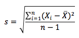
The sample standard deviation can be calculated by taking the square root of the sample variance. The sample standard deviation, s, is defined as :
The sample standard deviation can be calculated by taking the square root of the sample variance. The sample standard deviation, s, is defined as :
H. Calculate and interpret the proportion of observations falling within a specified number of standard deviations of the mean using Chebyshev's inequality :
Chebyshev’s inequality states that for any set of observations, whether sample or population data and regardless of the shape of the distribution, the percentage of the observations that lie within k standard deviations of the mean is at least 1 – 1/k2 for all k>1.
According to Chebyshev’s inequality, the following relationship hold true for any distribution. At least (1 – 1/k2) of observations lie within +/- k standard deviations of the mean.
I. Calculate and interpret the coefficient of variation and the Sharpe ratio :
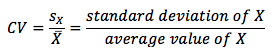
Relative dispersion is the amount of variability in a distribution relative to a reference point or benchmark. Relative dispersion is commonly measured with the coefficient of variation (CV), which is computed as :
CV measures the amount of dispersion in a distribution relative to the distribution’s mean. It is helpful because it enables us to make a direct comparison of dispersion across different sets of data. In an investment setting, the CV is used to measure the risk (variability) per unit of expected return (mean).
The Sharpe measure (Sharpe ratio or reward-to-variability ratio) is widely used for investment performance measurement and measures excess return per unit of risk. It is defined according to the following formula :
Chebyshev’s inequality states that for any set of observations, whether sample or population data and regardless of the shape of the distribution, the percentage of the observations that lie within k standard deviations of the mean is at least 1 – 1/k2 for all k>1.
According to Chebyshev’s inequality, the following relationship hold true for any distribution. At least (1 – 1/k2) of observations lie within +/- k standard deviations of the mean.
I. Calculate and interpret the coefficient of variation and the Sharpe ratio :
Relative dispersion is the amount of variability in a distribution relative to a reference point or benchmark. Relative dispersion is commonly measured with the coefficient of variation (CV), which is computed as :
CV measures the amount of dispersion in a distribution relative to the distribution’s mean. It is helpful because it enables us to make a direct comparison of dispersion across different sets of data. In an investment setting, the CV is used to measure the risk (variability) per unit of expected return (mean).
The Sharpe measure (Sharpe ratio or reward-to-variability ratio) is widely used for investment performance measurement and measures excess return per unit of risk. It is defined according to the following formula :
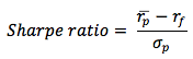
Notice that the numerator of the Sharpe ratio uses a measure for a risk-free return. As such, the quantity referred to as the excess return on portfolio P, measures the extra reward that investors receive for exposing themselves to risk. Portfolios with large positive Sharpe ratios are preferred to portfolios with smaller ratios because it is assumed that rational investors prefer return and dislike risk.
Analyst should be aware of two limitations of the Sharpe ratio : (1) If two portfolios have negative Sharpe ratios, it is not necessarily true that the higher Sharpe ratio implies superior risk-adjusted performance. (2) The Sharpe ratio is useful when standard deviation is an appropriate measure of risk. However, investment strategies with option characteristics have asymmetric return distributions, reflecting a large probability of small gains coupled with a small probability of large losses. In such cases, standard deviation may underestimate risk and produce Sharpe ratios that are too high.
J. Explain skewness and the meaning of a positively or negatively skewed return distribution :
A distribution is symmetrical if it is shaped identically on both sides of its mean. Distributional symmetry implies that intervals of losses and gains will exhibit the same frequency.
Skewness, or skew, refers to the extent to which a distribution is not symmetrical. Nonsymmetrical distributions may be either positively or negatively skewed and result from the occurrence of outliers in the data set. Outliers are observations with extraordinary large values, either positive or negative.
K. Describe the relative locations of the mean, median, and mode for unimodal, nonsymmetrical distribution :
Skewness affects the location of the mean, median, and mode of a distribution.
L. Explain measures of sample skewness and kurtosis :
Kurtosis is a measure of the degree to which a distribution is more or less “peaked” than a normal distribution. Leptokurtic describes a distribution that is more peaked (fat tails)than a normal distribution, whereas platykurtic refers to a distribution that is less peaked, or flatter than a normal distribution. A distribution is mesokurtic if it has the same kurtosis as a normal distribution.
A distribution is said to exhibit excess kurtosis if it has either more or less kurtosis than the normal distribution. The computed kurtosis for all normal distribution is three. Thus a normal distribution has excess kurtosis equal to zero, leptokurtic distribution has excess kurtosis greater than zero, and platykurtic distributions will have excess kurtosis less than zero.
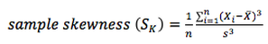
Sample skewness is computed as :
where s is sample standard deviation.
When a distribution is right skewed, sample skewness is positive and a left skewed distribution has a negative sample skewness.
Sample kurtosis is measured as :
Analyst should be aware of two limitations of the Sharpe ratio : (1) If two portfolios have negative Sharpe ratios, it is not necessarily true that the higher Sharpe ratio implies superior risk-adjusted performance. (2) The Sharpe ratio is useful when standard deviation is an appropriate measure of risk. However, investment strategies with option characteristics have asymmetric return distributions, reflecting a large probability of small gains coupled with a small probability of large losses. In such cases, standard deviation may underestimate risk and produce Sharpe ratios that are too high.
J. Explain skewness and the meaning of a positively or negatively skewed return distribution :
A distribution is symmetrical if it is shaped identically on both sides of its mean. Distributional symmetry implies that intervals of losses and gains will exhibit the same frequency.
Skewness, or skew, refers to the extent to which a distribution is not symmetrical. Nonsymmetrical distributions may be either positively or negatively skewed and result from the occurrence of outliers in the data set. Outliers are observations with extraordinary large values, either positive or negative.
- A positively skewed distribution is characterized by many outliers in the upper region, or right tail. A positively skewed distribution is said to be skewed right because of its relatively long upper right tail.
- A negatively skewed distribution is characterized by disproportionately large amount of outliers in the lower region, or left tail. A negatively skewed distribution is said to be skewed left because of its long lower tail.
K. Describe the relative locations of the mean, median, and mode for unimodal, nonsymmetrical distribution :
Skewness affects the location of the mean, median, and mode of a distribution.
- For a symmetrical distribution, the mean, median and mode are equal.
- For a positively skewed, unimodal distribution, the mode is less than the median, which is less than the mean.
- For a negatively skewed, unimodal distribution, the mean is less than the median, which is less than the mode.
L. Explain measures of sample skewness and kurtosis :
Kurtosis is a measure of the degree to which a distribution is more or less “peaked” than a normal distribution. Leptokurtic describes a distribution that is more peaked (fat tails)than a normal distribution, whereas platykurtic refers to a distribution that is less peaked, or flatter than a normal distribution. A distribution is mesokurtic if it has the same kurtosis as a normal distribution.
A distribution is said to exhibit excess kurtosis if it has either more or less kurtosis than the normal distribution. The computed kurtosis for all normal distribution is three. Thus a normal distribution has excess kurtosis equal to zero, leptokurtic distribution has excess kurtosis greater than zero, and platykurtic distributions will have excess kurtosis less than zero.
Sample skewness is computed as :
where s is sample standard deviation.
When a distribution is right skewed, sample skewness is positive and a left skewed distribution has a negative sample skewness.
Sample kurtosis is measured as :
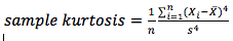
To interpret kurtosis, note that it is measured relative to the kurtosis of a normal distribution, which is 3 (excess kurtosis = sample kurtosis -3).
M. Compare the use of arithmetic and geometric means when analyzing investment returns :
Since past annual returns are compounded each period, the geometric mean of past annual returns is the appropriate measure of past performance. It gives us the average annual compound return.
The arithmetic mean is however the statistically best estimator of the next year’s returns given only the three years of return outcomes.
To estimate multi-year returns (next x years), the geometric mean is the appropriate measure.
|
|
